Kalman and Bayesian Filters in Python

Chapter 1 – The g-h Filter

1.1 Building Intuition via Thought Experiments

Imagine that we live in a world without scales – the devices you stand on to weigh yourself. One day at work a co-worker comes running up to you and announces her invention of a ‘scale’ to you. After she explains, you eagerly stand on it and announce the results: “172 lbs”. You are ecstatic – for the first time in your life you know what you weigh. More importantly, dollar signs dance in your eyes as you imagine selling this device to weight loss clinics across the world! This is fantastic!

Another co-worker hears the commotion and comes over to find out what has you so excited. You explain the invention and once again step onto the scale, and proudly proclaim the result: “161 lbs.” And then you hesitate, confused.

“It read 172 lbs a few seconds ago”, you complain to your co-worker.
“I never said it was accurate,” she replies.

Sensors are inaccurate. This is the motivation behind a huge body of work in filtering, and solving this problem is the topic of this book. I could just provide the solutions that have been developed over the last half century, but these solutions were developed by asking very basic, fundamental questions into the nature of what we know and how we know it. Before we attempt the math, let’s follow that journey of discovery, and see if it informs our intuition about filtering.

Try Another Scale 

Is there any way we can improve upon this result? The obvious, first thing to try is get a better sensor.

Unfortunately, your co-worker informs you that she has built 10 scales, and they all operate with about the same accuracy. You have her bring out another scale, and you weigh yourself on one, and then on the other. The first scale (A) reads “160 lbs”, and the second (B) reads “170 lbs”. What can we conclude about your weight?

Well, what are our choices?

• We could choose to only believe A, and assign 160lbs to our weight estimate.
• We could choose to only believe B, and assign 170lbs to our weight.
• We could choose a number less than both A and B.
• We could choose a number greater than both A and B.
• We could choose a number between A and B.

The first two choices are plausible, but we have no reason to favor one scale over the other. Why would we choose to believe A instead of B? We have no reason for such a belief. The third and fourth choices are irrational. The scales are admittedly not very accurate, but there is no reason at all to choose a number outside of the range of what they both measured. The final choice is the only reasonable one. If both scales are inaccurate, and as likely to give a result above my actual weight as below it, more often than not the answer is somewhere between A and B.

In mathematics this concept is formalized as expected value, and we will cover it in depth later. For now ask yourself what would be the ‘usual’ thing to happen if we took one million readings. Some of the times both scales will read too low, sometimes both will read too high, and the rest of the time they will straddle the actual weight. If they straddle the actual weight then certainly we should choose a number between A and B. If they don’t straddle then we don’t know if they are both too high or low, but by choosing a number between A and B we at least mitigate the effect of the worst measurement. For example, suppose our actual weight is 180 lbs. 160 lbs is a big error. But if we choose a weight between 160 lbs and 170 lbs our estimate will be better than 160 lbs. The same argument holds if both scales returned a value greater than the actual weight.

We will deal with this more formally later, but for now I hope it is clear that our best estimate is the average of A and B.

(160 + 170)/2 = 165

We can look at this graphically. I have plotted the measurements of A and B with an assumed error of ± 8 lbs. The measurements falls between 160 and 170 so the only weight that makes sense must lie within 160 and 170 lbs.

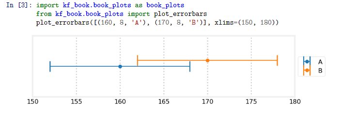
A word on how I generated this plot. I import code from the module book_plots in the kf_book subdirectory. Generating this plot takes a lot of boilerplate Python that isn’t interesting to read. I take this tack often in the book. When the cell is run plot_errorbars() gets called and the plot is inserted into the book.

If this is your first time using Jupyter Notebook, the code above is in a cell. The text “In [2]:” labels this as a cell where you can enter input, and the number in the bracket denotes that this cell was run second. To run the cell, click on it with your mouse so that it has focus, then press CTRL+ENTER on the keyboard. As we continue you will be able to alter the code inside the cells and rerun them. Try changing the values “160”, “170”, and “8” to some other value and run the cell. The printed output should change depending on what you entered.