Introduction to Statistical Thought

Chapter 1 – Probability

1.1 Basic Probability

Let X be a set and F a collection of subsets of X. A probability measure, or just a probability, on (X,F ) is a function µ : F → [0, 1]. In other words, to every set in F , µ assigns a probability between 0 and 1. We call µ a set function because its domain is a collection of sets. But not just any set function will do. To be a probability µ must satisfy

1. µ(∅) = 0 (∅ is the empty set.),
2. µ(X) = 1, and
3. if A1 and A2 are disjoint then µ(A1 ∪ A2) = µ(A1) + µ(A2).

One can show that property 3 holds for any finite collection of disjoint sets, not just two; see Exercise 1. It is common practice, which we adopt in this text, to assume more — that property 3 also holds for any countable collection of disjoint sets.

When X is a finite or countably infinite set (usually integers) then µ is said to be a discrete probability. When X is an interval, either finite or infinite, then µ is said to be a continuous probability. In the discrete case, F usually contains all possible subsets of X. But in the continuous case, technical complications prohibit F from containing all possible subsets of X. See Casella and Berger [2002] or Schervish [1995] for details. In this text we deemphasize the role of F and speak of probability measures on X without mentioning F .

In practical examples X is the set of outcomes of an “experiment” and µ is determined by experience, logic or judgement. For example, consider rolling a six-sided die. The set of outcomes is {1, 2, 3, 4, 5, 6} so we would assign X ≡ {1, 2, 3, 4, 5, 6}. If we believe the die to be fair then we would also assign µ({1}) = µ({2}) = · · · = µ({6}) = 1/6. The laws of probability then imply various other values such as

µ({1, 2}) = 1/3
µ({2, 4, 6}) = 1/2
etc.

Often we omit the braces and write µ(2), µ(5), etc. Setting µ(i) = 1/6 is not automatic simply because a die has six faces. We set µ(i) = 1/6 because we believe the die to be fair.

We usually use the word “probability” or the symbol P in place of µ. For example, we would use the following phrases interchangeably:

• The probability that the die lands 1
• P(1)
• P[the die lands 1]
• µ({1})

We also use the word distribution in place of probability measure. The next example illustrates how probabilities of complicated events can be calculated

from probabilities of simple events.

Example 1.1 (The Game of Craps) Craps is a gambling game played with two dice. Here are the rules, as explained on the website www.online-craps-gambling.com/craps-rules.html.

For the dice thrower (shooter) the object of the game is to throw a 7 or an 11 on the first roll (a win) and avoid throwing a 2, 3 or 12 (a loss). If none of these numbers (2, 3, 7, 11 or 12) is thrown on the first throw (the Come-out roll) then a Point is established (the point is the number rolled) against which the shooter plays. The shooter continues to throw until one of two numbers is thrown, the Point number or a Seven. If the shooter rolls the Point before rolling a Seven he/she wins, however if the shooter throws a Seven before rolling the Point he/she loses.

Ultimately we would like to calculate P(shooter wins). But for now, let’s just calculate

P(shooter wins on Come-out roll) = P(7 or 11) = P(7) + P(11).

Using the language of page 1, what is X in this case? Let d1 denote the number showing on the first die and d2 denote the number showing on the second die. d1 and d2 are integers from 1 to 6. So X is the set of ordered pairs (d1, d2) or

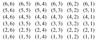
If the dice are fair, then the pairs are all equally likely. Since there are 36 of them, we assign P(d1, d2) = 1/36 for any combination (d1, d2). Finally, we can calculate

P(7 or 11) = P(6, 5) + P(5, 6) + P(6, 1) + P(5, 2) + P(4, 3) + P(3, 4) + P(2, 5) + P(1, 6) = 8/36 = 2/9.

The previous calculation uses desideratum 3 for probability measures. The different pairs (6, 5), (5, 6), . . . , (1, 6) are disjoint, so the probability of their union is the sum of their probabilities.

Example 1.1 illustrates a common situation. We know the probabilities of some simple events like the rolls of individual dice, and want to calculate the probabilities of more complicated events like the success of a Come-out roll. Sometimes those probabilities can be calculated mathematically as in the example. Other times it is more convenient to calculate them by computer simulation. We frequently use R to calculate probabilities. To illustrate, Example 1.2 uses R to calculate by simulation the same probability we found directly in Example 1.1.